This blogpost is dedicated to a simple and fast Rust based implementation of a quantum circuits emulator. The repository with a code of the emulator is accessible via the link, the entire code contains a lot of minor technical details that I do not discuss here, however I tried to cover all the crucial points forming the holistic picture. The first question that arises is why do we need to use Rust as a core language? Why don’t we use python frameworks such Jax or Julia language that are equipped with an easy parallelism, a jit compilation, and designed for efficient scientific computing? Let us discuss this question in details now.
Why Rust?
Rust is a system programming language that includes several strong advantages at once. It maintains zero-cost abstraction principle and minimal runtime without garbage collector as C/C++ and also has the same performance as C/C++. Meanwhile it is almost impossible to get undefined behaviour (UB) at runtime until you do not use unsafe blocks in your code. This is because Rust compiler detects all potential sources of UB at compile time and does not compile code that in some conditions leads to UB. Rust is also thread safe. This means that you could implement all sorts of parallelism and concurrency without being afraid of data races. The list of Rust advantages is quite long and we are not going to discuss all of them in here. The most important for us are those that are already listed above.
Now let us discuss why these advantages allow one to implement a better state-vector emulator in comparison with Python/Julia based ones. First of all, a state-vector emulator core is essentially a matrix-matrix multiplication module with some specific features:
- typically it is a multiplication of a small matrix with a very long and narrow one. In case of two-qubit gate it is a multiplication of a matrix of size \(4 \times 4\) (gate matrix) with a matrix of size \(4\times 2^{(n-2)}\) (state), where \(n\) is the number of qubits;
- it requires to use non-trivial slicing of a state, because you may apply a two-qubit gate to an arbitrary pair of quantum state qubits. It is not enough to maintain a row major and a column major matrix layouts or even matrix layouts with arbitrary strides.
Thus, one can take advantage from the purely custom implementation of this matrix-matrix multiplication. For example, it would be profitable to have the following features in our custom implementation:
- keep only one heap allocated buffer for the state vector and update it in-place;
- keep all gates on a stack;
- organize parallel and efficient traversal of the state vector without changing its memory layout.
These features require a low-level control of resources, minimal runtime, abstractions with clear memory layout and absence of hidden indirections. Meanwhile, it would be nice to have a compiler that prevents most of the safety bugs going together with low-level control at the compile time. Finally, the fearless parallelism together with easy to use and fast iterators provided by Rust are also very helpful. As one can see, Rust serves as a nice candidate to be the core language for such kind of things. Now, let us dive into the implementation.
Quantum state and its memory layout
The most important abstraction of the emulator is the quantum state. Quantum state of a system containing $n$ qubits is seen as a complex valued tensor with $n$ indices, where each index takes either $0$ or $1$. We need to have a fast access to an arbitrary element of the quantum state by its indices, therefore, the best data structure for this purpose is a contiguous heap allocated memory block (array) of an appropriate size. We also need some additional information about a quantum state stored together with this block. In Rust one can define the structure that fits all this requirements as follows:
struct QState<T: Float + Clone + Default + Sync + Send> {
    state: Vec<Complex<T>>,
    qubits_number: usize,
    task_size: usize,
}
As one can see T is a generic type that must be a cloneable floating point number, must have a default initializer and must be sync and send for multithreading purposes. The first field of the structure is the state itself. It is a vector (contiguous heap allocated buffer) with elements of type Complex<T>, i.e. complex numbers built on top of a type T. The second field is the number of qubits that corresponds to the size of the state buffer. The necessity of the third field will be clear further in the text, where we discuss the parallelization scheme. It is the size of a task that is sent to a particular thread.
Elements of Vec<Complex<T>> are accessible by a single index of type usize. But how can one access an element of the state via a multi-index \((i_0, i_1,\dots,i_{n-1})\), where \(i \in \{0, 1\}\), representing a particular basis element? This is done via the following natural transition from a multi-index to the corresponding single index
$I = \sum_{k=0}^{n-1} 2^k i_k$. Note, that conversion between single index and multi-index is the conversion between decimal and binary representations of the corresponding usize defining the index. We will take advantage of it in the next subsection.
Two-qubit operations: indices traversal
Now let us discuss how one can apply a quantum gate to a state defined above. We focus our attention on the two-qubit case, the downgrade to the one-qubit case is straightforward. Let us define an input quantum state as $S$ and an output quantum state as $\tilde{S}$. Elements of a state $\tilde{S}$ that is obtained by application of a two-qubit gate to qubits number $q$ and $p$ of a state $S$ may be represented by the following sum: \(\tilde{S}[i_0 + 2i_1 + \dots + 2^qi_q + \dots + 2^pi_p + \dots + 2^{n-1}i_{n-1}] \\= \sum_{i'_q, i'_p}U[8i_q + 4i_p + 2i'_q + i'_p]\\\cdot S[i_0 + 2i_1 + \dots + 2^qi'_q + \dots + 2^pi'_p + \dots + 2^{n-1}i_{n-1}],\) where $U$ is a two-qubit gate also stored in a contiguous memory block on a stack. This expression can be rewritten as follows:
\(\tilde{S}[2^qi_q + 2^pi_p + J] = \sum_{i'_q, i'_p}U[8i_q + 4i_p + 2i'_q + i'_p]S[2^qi'_q + 2^pi'_p + J]\), where by a single index $J$ we denote the expression that does not contain binary indices taking part in the summation. To evaluate this summation efficiently, one needs to be able to efficiently iterate over all possible values of $J$. To do that, let us take advantage of bitwise operations. $J$ takes $2^{(n-2)}$ usize values, almost all in a row starting from $0$ and skipping those which have $0$ at positions $i_q$ and $i_p$ in the binary representation of $J$. In order to iterate over all possible values of $J$, one simply needs to iterate over all values from the interval $[0, 2^{n-2})$ in a row and insert zeros at positions $i_q$ and $i_p$ in the binary representation of each value from the interval. This could be done via bitwise operations performed over usize type. Let us consider the following illustration that explains how one can do this:
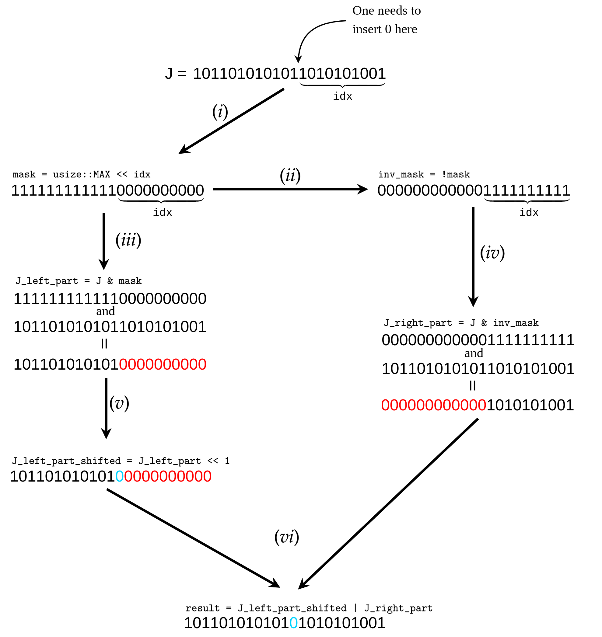 Let us say that we want to insert zero at position
 idx of the binary representation of J. Then, the overall procedure illustrated in the figure above is splitted into the six following steps:
- (i) We initialize a
maskvariable of typeusize, whose binary representation starts fromidxzeros and contains ones in the remaining part. I.e. it is initialized as followslet mask = usize::MAX << idx;; - (ii) We initialize a NOT version of
mask, namelyinv_mask, whose zeros and once of the binary representation are flipped. I.e. it is initialized as followslet inv_mask = !mask;; - (iii) We applies
masktoJ, i.e. take&(logical and) operation between them. This zeroes the right part of $J$. The result we store in an auxiliary variableJ_left_part, whose initialization readslet J_left_part = mask & J;; - (iv) The same we do with
inv_maskandJgettingJ_right_partthat readslet J_right_part = inv_mask & J;; - (v) We perform one bit right shift of the binary representation of
J_left_partin order to get the insertion of zero in the final result. The shifted version ofJ_left_partreadslet J_left_part_shifted = J_left_part << 1; - (vi) We take a logical or operation between
J_left_part_shiftedandJ_right_partas followslet result = J_left_part_shifted | J_right_part;obtaining the final result.
This algorithm is an illustration of what happens in the code, however, the logic of the algorithm is distributed between several abstractions. First abstraction is a function that takes a binary mask and index (value of $J$) and returns the value of $J$ with inserted zero in the binary representation according to the mask. This function reads:
fn insert_zero(idx: usize, mask: usize) -> usize {
  ((mask & idx) << 1) | ((!mask) & idx)
}
Second abstraction is the iterator whose definition and implementation is given below
struct Q2IdexIterator {
  mask1: usize,
  mask2: usize,
  state: usize,
  end: usize,
}

impl Q2IdexIterator {
  fn new(
    idx1: usize,
    idx2: usize,
    start: usize,
    len: usize,
  ) -> Self {
    let (min_idx, max_idx) = (std::cmp::min(idx1, idx2), std::cmp::max(idx1, idx2));
    Q2IdexIterator {
      mask1: usize::MAX << min_idx,
      mask2: usize::MAX << max_idx,
      state: start,
      end: len + start,
    }
  }
}
where Q2 part of a name means that this is an index iterator for the case of two-qubit operations.
It includes binary masks responsible for the insertion of two zeros into the binary representation, starting value and the length (total number of iteration) of the iterator. Since it is an iterator, it implements Iterator trait as it is shown below:
impl Iterator for Q2IdexIterator {
  type Item = usize;
  fn next(&mut self) -> Option<Self::Item> {
      if self.state >= self.end {
        None
      } else {
        let curr_state = self.state;
        self.state += 1;
        Some(insert_zero(insert_zero(curr_state, self.mask1), self.mask2))
      }
  }
}
i.e. it simply iterates from start to start + len and insert two zeros into the binary representation of each value when returns. Now we have a tool allowing us to not only traverse ``free’’ indices of a state efficiently but also split the overall summation into several tasks and perform them in parallel withing several threads. We discuss splitting into tasks in the next section.
Two-qubit operations: splitting the overall job into tasks
One can split the overall summation into smaller tasks, where each task performs a small piece of the job. It is convenient to define a separate structure for a task as follows:
pub struct Q2Task<'a, T: 'a>
{
  index_iter: Q2IdexIterator,
  mut_ptr: *mut Complex<T>,
  stride1: usize,
  stride2: usize,
  phantom: PhantomData<&'a T>,
}
Let us discuss each field of this structure in detail. First field is an iterator that iterates over $J$. It should not cover the entire set of possible values of $J$, typically it covers only a small part that forms a task. The second field is a mutable raw pointer to the beginning of the buffer that stores a quantum states. You may ask a question: Why do we need to use raw pointers? Their validity is not checked by the compiler, they require unsafe blocks for dereferencing and pointer arithmetics that may lead to the undefined behavior. Is it better to use a mutable reference? Unfortunatelly, with use of mutable references we are allowed to create and operate with only one task at a moment since mutable reference is unique. You may argue then: but by creating a several mutable pointers to the same object we violate all the safety rules, by passing them to several different threads we immediately fall into data race. Do not worry, we design our API in such a way, that it is impossible to access the same elements of a state from different tasks. Moreover, each task could be used and generated only once. The overall API remains safe after all. We will be accessing only different elements of a state from different threads. Third and fourth fields are strides for indices that are convolved with a two-qubit gate. I.e. the full traversal of a state can be implemented as follows:
for i in 0..2 {
  for j in 0..2 {
      index_iter.for_each(|J| {
          let item = state[J + i * stride1 + j * stride2]
          /* some code processing item */
      });
  }
}
this is an example that serves only for illustrative purposes to unravel the meaning of stride1 and stride2. The last field is needed to show that an object of type Q2Taks must not outlive a state, since it contains a mutable pointer to it.
That is it, the information in Q2Task is enough to perform a two-qubit task for values of $J$ that are contained in index_iter. One can send a task to a particular thread and then perform job over those part of the state Q2Task it has access to. Let us implement the logic that a task is allowed to perform:
impl<T> Q2Task<'_, T>
where
  T: Copy + Float + Default
{
  pub(super) fn matvec_inplace(self, matrix: &[Complex<T>]) {
    for idx in self.index_iter {
      let mut temp_arr: [Complex<T>; 4] = Default::default();
      for i in 0..2 {
        for j in 0..2 {
          for k in 0..2 {
            for l in 0..2 {
              unsafe {
                temp_arr[2 * i + j] = temp_arr[2 * i + j] + matrix[8 * i + 4 * j + 2 * k + l]
                                      * (*self.mut_ptr.add(self.stride1 * k + self.stride2 * l + idx));
              };
            }
          }
        }
      }
      for k in 0..2 {
        for l in 0..2 {
          unsafe {
            *self.mut_ptr.add(self.stride1 * k + self.stride2 * l + idx) = temp_arr[2 * k + l];
          };
        }
      }
    }
  }
}
The method matvec_inplace takes a two-qubit gate allocated on a stack, and performs in-place application of this gate to a part of a state. It allocates a temporal small buffer temp_arr on a stack for the result of a matrix-vector multiplication implemented as a set of nested loops and then write result from temp_arr back to a state. It performs this for all values of $J$ a Q2Task has access to. Note, that the method matvec_inplace takes a Q2Task by value, it means that Q2Task is being destructed after calling the method and can’t be used more than once. Now its time to discuss how exactly we split the entire job into tasks.
Two-qubit operations: tasks generation
One needs an abstraction that generates non-overlapping tasks that cover the entire job. A perfect candidate for such an abstraction is a structure that implements trait Iterator generating objects of type Q2Task. Let us define this structure as follows:
struct Q2TasksIterator<'a, T>
where
  T: Float + 'a,
{
  idx1: usize,
  idx2: usize,
  stride1: usize,
  stride2: usize,
  task_size: usize,
  state: usize,
  end: usize,
  mut_ptr: *mut Complex<T>,
  phantom: PhantomData<&'a mut T>,
}
This structure contains a lot of fields, let us discuss all of them one by one. First two fields are just indices that are convolved with a two-qubit gate. The next two fields are strides that are the same as for Q2Task. Field task_size is the number of different values of $J$ that are covered by a single generated Q2Task. Field state is the current state of a Q2TasksIterator whose actual meaning is the index that is starting index of the next generated Q2Task. Field end indicates the termination state of Q2TasksIterator. As for Q2Task field mut_ptr is a mutable raw pointer pointing to the beginning of the buffer where a quantum state is stored. The last field phantom as in case of Q2Task indicates that the structure must not outlive a quantum state.
Now let us have a look on the implementation of the Iterator trait for Q2TasksIterator:
impl<'a, T> Iterator for Q2TasksIterator<'a, T>
where
  T: Float + 'a,
{
  type Item = Q2Task<'a, T>;
  fn next(&mut self) -> Option<Self::Item> {
    if self.state >= self.end {
      None
    } else {
      let task_start = self.state;
      self.state += self.task_size;
      let task_index_iter = Q2IdexIterator::new(self.idx1, self.idx2, task_start, self.task_size);
      Some(Q2Task {
        index_iter: task_index_iter,
        mut_ptr: self.mut_ptr,
        stride1: self.stride1,
        stride2: self.stride2,
        phantom: PhantomData,
      })
    }
  }
}
As one can see, the method next updates the state of Q2TasksIterator by adding the task_size to it and creates Q2Task that covers the corresponding pice of a job. By iterating over Q2TasksIterator until exhaustion we get a set of Q2Task covering the entire quantum state. By calling the matvec_inplace on each Q2Task we update the entire state. Now let us have a look on how this job is distributed across threads.
Two-qubit operations: parallel tasks execution
In this section we consider a method apply_2q_gate of the QState structure that implements a parallel application of a two-qubit gate to a quantum state. The code of the method is given below:
fn apply_2q_gate(
    &mut self,
    gate: &[Complex<T>],
    idx1: usize,
    idx2: usize,
  )
  {
    let threads_number = self.threads_number;
    let task_iter = Q2TasksIterator::new(self, idx1, idx2, self.task_size);
    let(sn, rs) = bounded::<Q2Task<T>>(threads_number);
    scope(|s| {
      for _ in 0..threads_number {
        let local_rs = rs.clone();
        let gate_ref = &gate[..];
        s.spawn(move |_| {
          loop {
            let task = local_rs.recv();
            match task {
              Result::Err(..) => { break },
              Ok(q2task) => {
                q2task.matvec_inplace(gate_ref);
              },
            };
          }
        });
      }
      task_iter.for_each(|x| {
        sn.send(x).unwrap();
      });
      drop(sn);
    }).unwrap();
  }
let us discuss this method in detail. First of all, one gets number of threads from self and creates a Q2TasksIterator that will be generating tasks. Then, one create a crossbeam channel as follows let(sn, rs) = bounded::<Q2Task<T>>(threads_number);, where sn is a sender and rs is a receiver. Sender and receiver could be cloned and distributed across different threads. They share access to a single queue, any thread can push a task to a queue via its own copy of sn and any thread can pop a task from a queue via its own copy of rs. Therefore, a channel would be useful to send tasks to different threads. Next, one creates a number of threads using crossbeam scope. Each thread runs an infinite loop where it tries to read from its local copy of ‘rs’. When it receives a Q2Task it executes this task by running matvec_inplace. If it receives an error, it brakes the loop and the execution of a thread is stopped. After spawning threads, one runs a loop over task_iter where all tasks generated by the task_iter are being sent to sn, i.e. to the queue of tasks each spawned thread has access to. When all the tasks are sent to the channel, one drops sn closing the channel: when queue is empty, all threads receive an error and stop execution. That is it, one has a custom thread pool and a queue with tasks that are popped by free threads from a pool.
The implementation of the emulator contains a lot of smaller technical details that I do not explain here since they are not important for the general understanding of how the emulator works. For instance, I omitted the discussion of one-qubit operations, that include calculation of a one-qubit density matrix and application of a one-qubit gate to a quantum state, because they are analogous to two-qubit operations. For more details I refer a reader to the GitHub repo. Now let us discuss some numerical experiments and benchmarks of the emulator.
Quantum fourier transform
To roughly understand the performance of the obtained emulator I performed quantum Fourier transform (QFT) for different numbers of qubits. All the experiments were run on a laptop with the following CPU: 11th Gen Intel(R) Core(TM) i7-11800H @ 2.30GHz and 32GB of RAM. The following result was obtained for a single run of QFT for each number of qubits:
Total computation time for 10 qubits is 0.0149343 secs
Total computation time for 14 qubits is 0.0235194 secs
Total computation time for 18 qubits is 0.0584518 secs
Total computation time for 22 qubits is 0.8747207 secs
Total computation time for 26 qubits is 21.7860507 secs
Total computation time for 28 qubits is 106.9371843 secs
Total computation time for 30 qubits is 502.4312893 secs
Dynamics of 2D Quantum Heisenberg model
Of corse, one can use such an emulator not only to emulate quantum computations, but also to simulate dynamics of different quantum systems. To demonstrate this, I simulated dynamics of $5\times 5$ 2D Quantum Heisenberg model with zero external magnetic field, coupling parameter $J = 1$ and periodic boundary conditions. To do that, I represented the dynamics as a quantum circuit consisting of two-qubit gates. It is possible with use of trotterization. As discretization step I took $\tau = 0.03$, the total number of gate layers was equal to $200$ which corresponds to the total dynamics observation time $T = 6$. As an initial state of the model I took all spins pointing up except the middle spin pointing down. The following gif shows how the projection of each spin on $z$ axis ($z$ component of the Bloch vector of each individual spin) evolves in time:
Conclusion
Rust programming language is amazing. It allows one to implement fast and reliable programs for numerical simulation of complex systems with ease. Of corse, it is not as simple as with Julia or Python, but Rust proposes much more possibilities since you may implement almost anything from scratch without any performance trade-off.
Feel free to modify the code from the repo for your purposes. The core logic of the emulator is placed in the folder state_vector_machine, you can apply it to your own numerical experiments.